Usage

Audio File

To turn an audio file into an OSEkit AudioFile (represented by the osekit.core_api.audio_file.AudioFile class), all you need is the path to the file and a begin timestamp.

Such begin timestamp can either be specified (as a pandas.Timestamp instance), or parsed from the audio file name by specifing the strptime format:

from osekit.core_api.audio_file import AudioFile
from pathlib import Path

af = AudioFile(
    path = Path(r"foo/7189.230405154906.wav"),
    strptime_format = "%y%m%d%H%M%S",
    )

Audio Data

Design

The osekit.core_api.audio_data.AudioData class represent a chunk of audio taken between two specific timestamps from one or more AudioFile instances.

This class offers means of easily resample the data and access it on-demand (with an optimized I/O workflow to minimize the file openings/closings).

To create an AudioData from AudioFiles, use the osekit.core_api.audio_data.AudioData.from_files() class method.

Example for an AudioData representing the first 2 seconds of the foo/7189.230405154906.wav audio file:

from pandas import Timestamp, Timedelta
from osekit.core_api.audio_data import AudioData

ad = AudioData.from_files(
files=[af],
end=af.begin + Timedelta(seconds=2) # begin and end defaults to the files boundaries: this will take the 2 first seconds of the audio file.
)

This will lead to the following data <-> file structure (see the Data and Files section):

If the AudioData begin and end timestamps cover multiple AudioFile, the corresponding AudioItem.

For example, the foo folder here below contains 4 10 s-long files, with a 10 s gap between the 3rd and 4th files:

foo
├── 7189.230405154906.wav
├── 7189.230405154916.wav
├── 7189.230405154926.wav
└── 7189.230405154946.wav

Let’s create a single AudioData that covers the total duration of the 4 files:

afs = [
    AudioFile(f, strptime_format="%y%m%d%H%M%S")
    for f in foo.glob("*.wav")
    ]

ad = AudioData.from_files(files=afs) # begin and end to default will cover the whole duration of the files

This will create one AudioItem per file, plus one empty AudioItem for the gap:

We can check that with code:

>>> print("\n".join("\n\t".join((f"Item {idx}", f"{f'Begin':<15}{str(item.begin):>20}", f"{f'End':<15}{str(item.end):>20}", f"{f'Is gap':<15}{"YES" if item.is_empty else "NO":>20}")) for idx,item in enumerate(sorted(ad.items, key=lambda i: i.begin))))
"""
Item 0
        Begin           2023-04-05 15:49:06
        End             2023-04-05 15:49:16
        Is gap                           NO
Item 1
        Begin           2023-04-05 15:49:16
        End             2023-04-05 15:49:26
        Is gap                           NO
Item 2
        Begin           2023-04-05 15:49:26
        End             2023-04-05 15:49:36
        Is gap                           NO
Item 3
        Begin           2023-04-05 15:49:36
        End             2023-04-05 15:49:46
        Is gap                          YES
Item 4
        Begin           2023-04-05 15:49:46
        End             2023-04-05 15:49:56
        Is gap                           NO
"""

Reading data

The osekit.core_api.audio_data.AudioData.get_value() method returns a numpy.ndarray that contains the wav values of the audio data.

The data is fetched seamlessly on-demand from the audio file(s). The opening/closing of the audio files is optimized thanks to a osekit.core_api.audio_file_manager.AudioFileManager instance.

Eventual time gap between audio items are filled with 0. values.

Calibration

The osekit.core_api.instrument.Instrument class can be used to provide calibration info to your audio data. This can be used to convert raw WAV data to the recorded acoustic pressure.

An Instrument instance can be attached to an AudioData. Then, the osekit.core_api.audio_data.AudioData.get_value_calibrated() method allows for retrieving the data in the shape of the recorded acoustic pressure.

from osekit.core_api.instrument import Instrument
from osekit.core_api.audio_data import AudioData
import numpy as np

instrument = Instrument(end_to_end_db = 150) # The raw 1. WAV value equals 150 dB SPL re 1 uPa
ad = AudioData(..., instrument=Instrument)

p = ad.get_value_calibrated()
spl = 20*np.log10(p/instrument.P_REF) # P_REF is 1 uPa by default

Resampling

AudioData can be resampled just by modifying the osekit.core_api.audio_data.AudioData.sample_rate field.

Modifying the sample rate will not access the data, but the data will be resampled on the fly when it is requested:

from osekit.core_api.audio_data import AudioData

ad = AudioData(...)
ad.sample_rate = 48_000 # Resample the signal at 48 kHz. Nothing happens yet
resampled_signal = ad.get_value() # The original audio data will be resampled while being fetched here.

Audio Dataset

The osekit.core_api.audio_dataset.AudioDataset class enables the instantiation and manipulation of large amounts of AudioData objects with simple operations.

Instantiation

The constructor of the AudioDataset class accepts a list of AudioData as parameter.

But this is not the only way to create an audio dataset. The osekit.core_api.audio_dataset.AudioDataset.from_folder() class method allows to easily instantiate an AudioDataset from a given folder containing audio files:

from pathlib import Path
from osekit.core_api.audio_dataset import AudioDataset
from pandas import Timestamp, Timedelta

folder = Path(r"...")
ads = AudioDataset.from_folder
(
    folder=folder,
    strptime_format="%y_%m_%d_%H_%M_%S", # To parse the files begin Timestamp
    begin=Timestamp("2009-01-06 12:00:00"),
    end=Timestamp("2009-01-06 14:00:00"),
    data_duration=Timedelta("10s")
)

The resulting AudioDataset will contain 10s-long AudioData ranging from 2009-01-06 12:00:00 to 2009-01-06 14:00:00.

This is the default behaviour, but other ways of computing the AudioData time locations are available through the osekit.core_api.audio_dataset.AudioDataset.from_folder() mode parameter (see the API documentation for more info).

You don’t have to worry about the shape of the original audio files: audio data will be fetched seamlessly in the corresponding file(s) whenever you need it.

Manipulation

If one wanted to resample these 10s-long audio data and export them as wav files, the AudioDataset makes it easy:

ads.sample_rate = 48_000 # The sample rate of all AudioData will be edited
ads.write(folder / "output") # All audio data will be exported to wav files in that folder

All the AudioData constituting the AudioDataset are accessible through the osekit.core_api.audio_dataset.AudioDataset.data field:

# Filtering the ads data to remove data without audio (e.g. between files)
ads.data = [ad for ad in ads.data if not ad.is_empty]

# Resampling/Exporting only the first audio data
ad = ads.data[0]
ad.sample_rate = 128_000
ad.write(folder / "alone_data")

Spectro Data

The osekit.core_api.spectro_data.SpectroData class allows to perform spectral computations and to plot spectrograms from AudioData objects.

The most straightforward way to instantiate a SpectroData is from an AudioData and a scipy.signal.ShortTimeFFT instance:

from osekit.core_api.audio_data import AudioData
from osekit.core_api.spectro_data import SpectroData
from scipy.signal import ShortTimeFFT
from scipy.signal.windows import hamming

ad = AudioData(...) # See AudioData documentation

sft = ShortTimeFFT(
    win=hamming(1024),
    hop=512,
    fs=ad.sample_rate,
)

sd = SpectroData.from_audio_data(data=ad, fft=sft)

Once again, no audio has yet been fetched: everything happens only on-demand.

NPZ matrices

The SpectroData object can be used to compute the spectrum matrices of the AudioData with the osekit.core_api.spectro_data.SpectroData.get_value() method.

The osekit.core_api.spectro_data.SpectroData.sx_dtype property can be set to either complex (default) or float to return either the spectrum matrices as complex numbers or absolute values, respectively.

The spectrum matrices can be converted to decibels thanks to the osekit.core_api.spectro_data.SpectroData.to_db() method. This method will convert the matrix values either to dB SPL (re Instrument.P_REF) if an Instrument was provided to the AudioData or to dB FS otherwise.

The spectrum matrices can then be exported to npz files thanks to the osekit.core_api.spectro_data.SpectroData.write() method.

sd = SpectroData.from_audio_data(data=ad, fft=sft)

sx = sd.get_value()
sx_db = sd.to_db(sx)

# If sx has already been computed, you can pass it as a parameter to avoid re-computing it.
# Otherwise, it will just be computed from scratch.
sd.write(Path(r"output_folder"), sx=sx)

Plot and export

Spectrograms can be plotted from the SpectroData objects thanks to the osekit.core_api.spectro_data.SpectroData.plot() method.

OSEkit uses pyplot for plotting spectrograms. A pyplot Axes can be provided to the SpectroData.plot() method to specify an Axes in which to plot the spectrogram:

from osekit.core_api.spectro_data import SpectroData
import matplotlib.pyplot as plt

sd = SpectroData(...) # See SpectroData documentation

sd.plot() # This will plot on a default figure
plt.show()

_, axs = plt.subplots(2,1)
sd.plot(ax=axs[0])
plt.show() # The spectrogram will be plotted on the top Axes of the figure

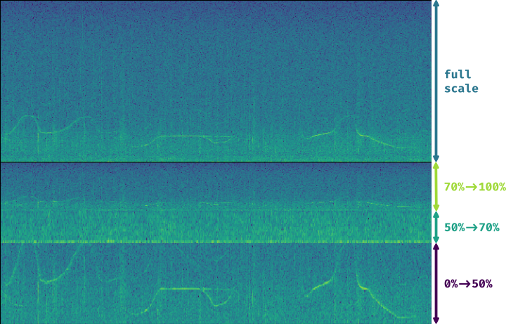
Custom frequency scales

The y-axis of the spectrograms can be parametrized thanks to the osekit.core_api.frequency_scale.Scale class.

The custom Scale is made of ScalePart (osekit.core_api.frequency_scale.ScalePart). Each ScalePart correspond to a given frequency range on a given area of the y-axis:

from osekit.core_api.frequency_scale import Scale, ScalePart

scale = Scale(
    [
        ScalePart(
            p_min=0., # From 0% of the axis
            p_max=.5, # To 50% of the axis
            f_min=5_000., # From 5 kHz
            f_max=20_000, # To 20 kHz
        ),
        ScalePart(
            p_min=.5, # From 50% of the axis
            p_max=.7, # To 70% of the axis
            f_min=0., # From 5 kHz
            f_max=3_000., # To 20 kHz
        ),
        ScalePart(
            p_min=.7, # From 70% of the axis
            p_max=1., # To 100% of the axis
            f_min=0., # From 0 Hz
            f_max=72_000, # To 72 kHz
        ),
    ],
)
fig, axs = plt.subplots(2,1)
sd.plot(ax=axs[0]) # We plot the full spectrogram at the top
sd.plot(ax=axs[1],scale=scale) # And the custom scale one at the bottom
plt.subplots_adjust(left=0, right=1, top=1, bottom=0, hspace=0, wspace=0)
plt.show()

The resulting figure presents the full-scale spectrogram at the top (from 0 to 72 kHz), and the custom-scale one at the bottom:

LTAS Data

OSEkit provides the osekit.core_api.ltas_data.LTASData class for computing and plotting LTAS (Long-Term Average Spectrum).

LTAS are suitable when a spectrum is computed over a very long time and that the spectrum matrix time dimension reach a really high value. In that case, time bins can be averaged to form a LTAS, which time resolution is lower than that of the original spectrum.

In OSEkit, LTAS are computed recursively: the user specifies a target number of time bins in the spectrum matrix, noted n_bins.

The visualization below depicts the process: the LTAS is computed with a target n_bins = 3000. Yellow rectangles depict the audio data (the x-axis being the time axis), and the number in the lower right corner depicts the number of time bins in the spectrum matrix for this audio data. The audio is recursively split in n_bins parts (it is split in 3 in the representation instead of 3000 for clarity purposes) until the number of time bins in the matrix gets below n_bins. Then, these spectrum parts are computed (hatched rectangles) and averaged across the time axis (filled rectangles).

LTASData objects inherit from SpectroData. It uses the same methods, only the additionnal nb_time_bins parameter should be provided:

ad = AudioData(...) # See AudioData documentation
sft = ShortTimeFFT(win = 1024, hop = 512, fs = ad.sample_rate)
ltas = LTASData.from_audio_data(data=ad, fft=sft, nb_time_bins=3000)

ltas.plot()
plt.show()

A SpectroData object can be turned into a LTASData thanks to the osekit.core_api.ltas_data.LTASData.from_spectro_data() method.