
Computing a LTAS with the Core API [1]#
Create an OSEkit AudioData from the files on disk.
There are multiple ways to achieve that, but the most straightforward is to use an AudioDataset that covers the whole time span of the files by leaving begin, end and data_duration at the None default value.
An Instrument can be provided to the AudioDataset for the WAV data to be converted in pressure units. This will lead the resulting spectra to be expressed in dB SPL (rather than in dB FS):
from pathlib import Path

audio_folder = Path(r"_static/sample_audio/timestamped")

from osekit.core.audio_dataset import AudioDataset
from osekit.utils.audio import Normalization
from osekit.core.instrument import Instrument

audio_data = AudioDataset.from_folder(
    folder=audio_folder,
    strptime_format="%y%m%d_%H%M%S",
    instrument=Instrument(end_to_end_db=150.0),
).data[0]

# Resampling at 24 kHz
audio_data.sample_rate = 24_000

# Removing the DC component
audio_data.normalization = Normalization.DC_REJECT
The AudioData object covers the whole time span of the audio files:
print(f"{' AUDIO DATASET ':#^60}")
print(f"{'Begin:':<30}{str(audio_data.begin):>30}")
print(f"{'End:':<30}{str(audio_data.end):>30}")
print(f"{'Sample rate:':<30}{str(audio_data.sample_rate):>30}")
###################### AUDIO DATASET #######################
Begin:                                   2022-09-25 22:34:50
End:                                     2022-09-25 22:36:50
Sample rate:                                           24000
Instantiate a scipy.signal.ShortTimeFFT FFT object with the required parameters:
from scipy.signal import ShortTimeFFT
from scipy.signal.windows import hamming

sft = ShortTimeFFT(
    win=hamming(1024),
    hop=128,  # This will be forced to len(win) if we compute a LTAS
    fs=audio_data.sample_rate,
)
Create an OSEkit SpectroDataset from the AudioDataset and the ShortTimeFFT objects:
from osekit.core.spectro_data import SpectroData

spectro_data = SpectroData.from_audio_data(
    data=audio_data,
    fft=sft,
    v_lim=(0.0, 150.0),  # Boundaries of the spectrogram
    colormap="viridis",  # Default value
)
Checking the required RAM to store the spectrum matrix can give a hint on when to switch to a LTAS computation:
print(f"{' SPECTRO DATA ':#^60}")
print(f"{'Matrix shape:':<30}{str(spectro_data.shape):>30}")
print(f"{'Matrix weight:':<30}{f'{str(round(spectro_data.nb_bytes / 1e6, 2))} MB':>30}")
####################### SPECTRO DATA #######################
Matrix shape:                                   (513, 22507)
Matrix weight:                                     184.74 MB
As displayed, the SX matrix has 22507 time bins.
Let’s turn the SpectroData object in a LTASData, where we will average time bins to force a given x-axis size (3000 in this example):
from osekit.core.ltas_data import LTASData

ltas_data = LTASData.from_spectro_data(
    spectro_data=spectro_data,
    nb_time_bins=3000,
)
The size and weight reduction can be checked:
print(f"{' LTAS DATA ':#^60}")
print(f"{'Matrix shape:':<30}{str(ltas_data.shape):>30}")
print(f"{'Matrix weight:':<30}{f'{str(round(ltas_data.nb_bytes / 1e6, 2))} MB':>30}")
######################## LTAS DATA #########################
Matrix shape:                                    (513, 3000)
Matrix weight:                                      12.31 MB
Now is time to compute the SX values of the LTAS (it can be stored in a variable so that it won’t be computed again when plotting or saving them):
ltas_sx = ltas_data.get_value()
We can now plot the LTAS:
import matplotlib.pyplot as plt

ltas_data.plot(sx=ltas_sx)
plt.show()
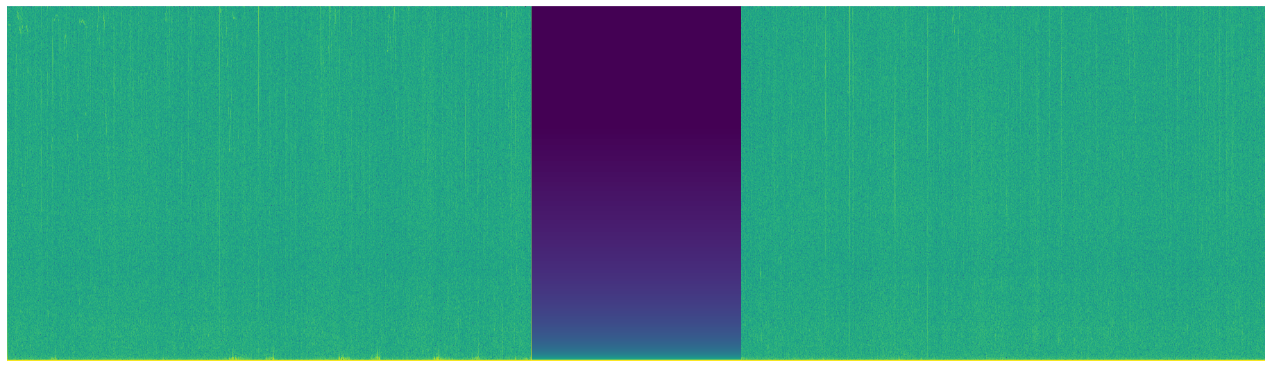
The time period in the middle where no audio has been recorded is clearly visible. Both the spectrogram and the sx matrix can be saved to disk:
# Export all spectrograms
ltas_data.save_spectrogram(folder=audio_folder / "spectrogram", sx=ltas_sx)

# Export all NPZ matrices
ltas_data.write(folder=audio_folder / "spectrum", sx=ltas_sx)