
Computing multiple spectrograms with the Public API [1]#
As always in the Public API, the first step is to build the project.
Since we don’t know (nor we care about) the files begin timestamps, we’ll set the striptime_format to None, which will assign a default timestamp at which the first valid audio file will be considered to start. Then, each next valid audio file will be considered as starting at the end of the previous one. This default timestamp can be editted thanks to the first_file_begin parameter.
An Instrument can be provided to the Project for the WAV data to be converted in pressure units. This will lead the resulting spectra to be expressed in dB SPL (rather than in dB FS).
from pathlib import Path

audio_folder = Path(r"_static/sample_audio/id")

from osekit.public.project import Project
from osekit.core.instrument import Instrument

project = Project(
    folder=audio_folder,
    strptime_format=None,
    instrument=Instrument(end_to_end_db=165.0),
)

project.build()
	2026-06-25 13:26:54,868
Building the project...
	2026-06-25 13:26:54,870
Analyzing original audio files...
	2026-06-25 13:26:54,875
Organizing project folder...
	2026-06-25 13:26:54,880
Build done!
The Public API Project is now analyzed and organized:
print(f"{' DATASET ':#^60}")
print(f"{'Begin:':<30}{str(project.origin_dataset.begin):>30}")
print(f"{'End:':<30}{str(project.origin_dataset.end):>30}")
print(f"{'Sample rate:':<30}{str(project.origin_dataset.sample_rate):>30}\n")

print(f"{' ORIGINAL FILES ':#^60}")
import pandas as pd

pd.DataFrame(
    [
        {
            "Name": f.path.name,
            "Begin": f.begin,
            "End": f.end,
            "Sample Rate": f.sample_rate,
        }
        for f in project.origin_files
    ],
).set_index("Name")
######################### DATASET ##########################
Begin:                                   2020-01-01 00:00:00
End:                                     2020-01-01 00:01:30
Sample rate:                                           48000

###################### ORIGINAL FILES ######################
| Begin | End | Sample Rate | |
|---|---|---|---|
| Name | |||
| 1829.wav | 2020-01-01 00:00:00 | 2020-01-01 00:00:10 | 48000 |
| 1830.wav | 2020-01-01 00:00:10 | 2020-01-01 00:00:20 | 48000 |
| 1832.wav | 2020-01-01 00:00:20 | 2020-01-01 00:00:30 | 48000 |
| 1833.wav | 2020-01-01 00:00:30 | 2020-01-01 00:00:40 | 48000 |
| 1834.wav | 2020-01-01 00:00:40 | 2020-01-01 00:00:50 | 48000 |
| 1835.wav | 2020-01-01 00:00:50 | 2020-01-01 00:01:00 | 48000 |
| 1836.wav | 2020-01-01 00:01:00 | 2020-01-01 00:01:10 | 48000 |
| 1837.wav | 2020-01-01 00:01:10 | 2020-01-01 00:01:20 | 48000 |
| 1838.wav | 2020-01-01 00:01:20 | 2020-01-01 00:01:30 | 48000 |
Since we will run a spectral transform, we need to define the FFT parameters:
from scipy.signal import ShortTimeFFT
from scipy.signal.windows import hamming

sample_rate = 24_000

sft = ShortTimeFFT(win=hamming(1024), hop=128, fs=sample_rate)
To run transforms in the Public API, use the Transform class:
from osekit.public.transform import Transform, OutputType
from osekit.utils.audio import Normalization

transform = Transform(
    OutputType.SPECTROGRAM,
    mode="files",  # We want one spectrogram per file
    sample_rate=sample_rate,
    normalization=Normalization.DC_REJECT,
    fft=sft,
    v_lim=(0.0, 150.0),  # Boundaries of the spectrograms
    colormap="viridis",  # Default value
    name="8s_long_spectros",
)
The Core API can still be used on top of the Public API.
We’ll access the Core API SpectroDataset that match this transform to trim and rename the exported spectrograms:
from pandas import Timedelta

spectro_dataset = project.prepare_spectro(transform)

for sd in spectro_dataset.data:
    sd.name = next(iter(sd.audio_data.files)).path.stem
    sd.end = sd.begin + Timedelta(seconds=8)
	2026-06-25 13:26:54,913
Creating the audio data...
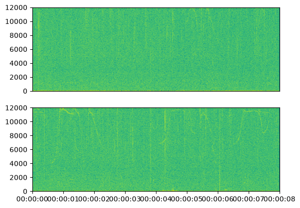
We can also glance at the spectrogram results with the Core API:
import matplotlib.pyplot as plt

fig, axs = plt.subplots(2, 1)
spectro_dataset.data[0].plot(ax=axs[1])
spectro_dataset.data[1].plot(ax=axs[0])
axs[0].get_xaxis().set_visible(False)

plt.show()
Running the transform while specifying the filtered audio_dataset will skip the empty AudioData (and thus the empty SpectroData).
project.run(transform=transform, spectro_dataset=spectro_dataset)
	2026-06-25 13:26:55,338
Creating the audio data...
	2026-06-25 13:26:55,343
Running transform...
	2026-06-25 13:26:55,343
Computing and writing spectrograms...
	2026-06-25 13:27:00,804
Transform done!
All the new files from the transform are stored in a SpectroDataset named after transform.name:
pd.DataFrame(
    [
        {
            "Exported file": path.name,
        }
        for path in (
            audio_folder / "processed" / transform.name / "spectrogram"
        ).iterdir()
    ],
).set_index("Exported file")
| Exported file |
|---|
| 1829.png |
| 1835.png |
| 1830.png |
| 1832.png |
| 1836.png |
| 1838.png |
| 1837.png |
| 1834.png |
| 1833.png |