
Using APLOSE detection results [1]#
Creating the Public Project#
APLOSE-compatible projects are build thanks to OSEkit’s Public API.
First, we will build a project and run a transform that would be uploaded and annotated on APLOSE (see the Public API documentation for more info).
The _static/detections/aplose_results.csv file used in this notebook simulates the results of this annotation campaign.
Build the Project#
First, we have to build the project from the raw audio files:
from pathlib import Path
from osekit.public.project import Project
from osekit.core.instrument import Instrument

folder = Path(r"_static/sample_audio/timestamped")
strptime_format = r"%y%m%d_%H%M%S"

project = Project(
    folder=folder,
    strptime_format=strptime_format,
    instrument=Instrument(end_to_end_db=150.0),
    timezone="UTC",
)

project.build()
	2026-09-28 15:47:34,740
Building the project...
	2026-09-28 15:47:34,741
Analyzing original audio files...
	2026-09-28 15:47:34,768
Organizing project folder...
	2026-09-28 15:47:34,773
Build done!
Declare & Run the Transform#
Then we declare and run a Transform which would export the spectrograms to be annotated:
from osekit.public.transform import Transform, OutputType
from osekit.utils.audio import Normalization
from pandas import Timestamp, Timedelta
from scipy.signal import ShortTimeFFT
from scipy.signal.windows import hamming

transform = Transform(
    output_type=OutputType.SPECTROGRAM,
    begin=Timestamp("2022-09-25 22:35:15+0000"),
    end=Timestamp("2022-09-25 22:36:25+0000"),
    data_duration=Timedelta(seconds=7.5),
    normalization=Normalization.DC_REJECT,
    fft=ShortTimeFFT(win=hamming(1024), hop=128, fs=project.origin_dataset.sample_rate),
    v_lim=(50.0, 120.0),  # Boundaries of the spectrograms
    colormap="viridis",  # Default value
    name="example_transform",
)

# We remove all spectrograms that contain silent parts
ads = project.prepare_audio(transform=transform)
ads.remove_empty_data(threshold=0.99)

project.run(transform=transform, audio_dataset=ads)
	2026-09-28 15:47:34,781
Creating the audio data...
	2026-09-28 15:47:34,794
Running transform...
	2026-09-28 15:47:34,795
Computing and writing spectrograms...
	2026-09-28 15:47:40,026
Transform done!
Parse the detection result csv file thanks to the Detection class:
from pathlib import Path
from osekit.core.detection import Detection

detections = Detection.from_csv(csv=Path(r"_static/detections/aplose_results.csv"))
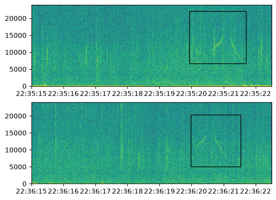
Filtering the detections#
We can use basic python filtering to access specific detections.
Here, we will:
Keep only
Odontocete whistledetections of typeBOXwith a strong confidence levelFilter the
SpectroDatasetto keep only the files in which such detections were madePlot the detections as
Rectangles on the spectrograms
Keeping specific detections#
Filtering out unwanted detections can be done with a basic list comprehension:
def does_satisfy_constraints(detection: Detection) -> bool:
    # Keeping only odontocete whistles
    if detection.label != "Odontocete whistle":
        return False

    # Keeping only BOX detections
    if detection.type != "BOX":
        return False

    # Keeping only maximum confidence level detections
    if (
        detection.confidence_indicator.level
        < detection.confidence_indicator.maximum_level
    ):
        return False

    return True


filtered_detections = [
    detection for detection in detections if does_satisfy_constraints(detection)
]
Filtering the SpectroDataset#
Detections inherit from the Event class, which allows for an easy filtering of the SpectroData:
# Recover the transform output (SpectroDataset)
sds = project.get_output(output_name="example_transform")

# Keeping only SpectroDatas that contain filtered detections
sds.data = [
    sd
    for sd in sds.data
    if any(detection.overlaps(sd) for detection in filtered_detections)
]
Plotting the Spectrograms along with detections#
We then want to plot detection boxes directly the spectrograms:
import matplotlib.pyplot as plt

# Create a figure with one spectrogram per row
fig, axs = plt.subplots(nrows=len(sds.data), ncols=1)

# Plot spectrograms
for idx, sd in enumerate(sds.data):
    # We want to plot each spectrogram in a specific ax
    ax = axs[idx]

    sd.plot(ax=ax)

    # We want to plot all detections related to this spectrogram
    for detection in filtered_detections:
        if not detection.overlaps(sd):
            continue

        # Detections are plotted as matplotlib Rectangles
        rectangle = detection.to_rectangle(fill=False)
        ax.add_patch(rectangle)

# Let's take a look at the output figure
plt.show()
# Reset the project to get all files back to place.
project.reset()